
Full Text View
Volume 20 Issue 4 (April-May 2010)
GSA Today
![]()
Article, pp. 4-10 | Abstract | PDF (3.4MB)
The digital revolution in geologic mapping
| Table of Contents |
|---|
|
Search GoogleScholar for
Search GSA Today |
Abstract
Geologic field data collection, analysis, and map compilation are undergoing a revolution in methods, largely precipitated by global positioning system (GPS) and geographic information system (GIS) equipped mobile computers paired with virtual globe visualizations. Modern, ruggedized personal digital assistants (PDAs) and tablet PCs can record a wide spectrum of geologic data and facilitate iterative geologic map construction and evaluation on location in the field. Spatial data, maps, and interpretations can be presented in a variety of formats on virtual globes, such as Google Earth and NASA World Wind, given only a basic knowledge of scripting languages. As a case study, we present geologic maps assembled in Google Earth that are based on digital field data. Interactive features of these maps include (1) the ability to zoom, pan, and tilt the terrain and map to any desired viewpoint; (2) selectable, draped polygons representing the spatial extent of geologic units that can be rendered semi-transparent, allowing the viewer to examine the underlying terrain; (3) vertical cross sections that emerge from the subsurface in their proper location and orientation; (4) structural symbols (e.g., strike and dip), positioned at outcrop locations, that can display associated metadata; and (5) other data, such as digital photos or sketches, as clickable objects in their correct field locations.
Google Earth–based interactive geologic maps communicate data and interpretations in a format that is more intuitive and easy to grasp than the traditional format of paper maps and cross sections. The virtual three-dimensional (3-D) interface removes much of the cognitive barrier of attempting to visualize 3-D features from a two-dimensional map or cross section. Thus, the digital revolution in geologic mapping is finally providing geoscientists with tools to present important concepts in an intuitive format understandable to the expert and layperson alike.
Manuscript received 27 July 2009; accepted 13 Oct. 2009
DOI: 10.1130/GSATG70A.1
E-mails: , ,
INTRODUCTION
The presentation of spatial geologic data as maps and cross sections essentially began with Cuvier and Brongniarts (1808) map of the Paris Basin and Smiths (1815) geologic map of England and Wales. Their approach to presenting field data as color-coded units in recognizable map formats became the de facto standard for geologists around the globe (e.g., Griffith, 1838; Hitchcock, 1878). These geologic maps were based on countless hours of classifying, measuring, cataloguing, and interpolating rock units across field areas at outcrop to continental scales. Over the years, the means of transportation for fieldwork advanced from horseback to four-wheel drive vehicles, but the basic methods of field data collection and presentation remained largely unchanged.
The first years of the twenty-first century saw a major advance in the methods of field data acquisition and geologic map presentation. This was facilitated by three main technological advances: (1) the descrambling of global positioning system (GPS) satellite signals, (2) the advent of affordable mobile computers capable of running geographic information system (GIS) software in the field, and (3) the universal availability of free, Web-based virtual globes (also known as digital globes or geobrowsers). Although GPS had been operational since the mid-1990s, it wasnt until 2000, when Selective Availability was discontinued, that GPS became effective as a precise positioning tool for the general populace (White House Office of Science and Technology Policy [OSTP], 2000). Manufacturers began producing inexpensive handheld and car-mounted GPS devices as backpacking and motorized travel aids. At the same time, computer manufacturers started marketing portable personal digital assistants (PDAs) and tablet PCs capable of integrating GPS with GIS software for mobile digital data collection. Today, advanced mobile computing systems, such as the Trimble Explorer series and xPlore tablet PCs, are ruggedized and water-resistant enough to handle the typical bumps, scratches, and rain showers common to geologic field mapping and research.
Techniques for the digital presentation of geologic maps advanced during the late twentieth century using an assortment of proprietary platforms (e.g.,Selner and Taylor, 1993; Condit, 1995). Recent developments utilize free and almost universally accessible global terrain models within Web-based virtual globes, such as NASA World Wind, Google Earth, and Microsoft Virtual Earth. These “geobrowsers” generally support the open-source scripting language KML (Keyhole Markup Language), an XML-derived language that facilitates user manipulation of a geobrowser environment. KML scripting has enabled geoscientists, as well as other producers of spatial data sets, to display field data and maps in a virtual three-dimensional (3-D) interface. Provided the user has an active, reasonably fast Internet connection, the possibilities for exploring an ever-expanding collection of geospatial data sets from locations around the globe are almost unlimited. Users can bypass the requirement for an active Internet connection by loading pertinent data and maps into the cache of a geobrowser, thereby enabling access to a virtual 3-D interface on location in the field.
This article documents an approach to geologic field mapping and presentation that utilizes recent technological and methodological advances and illustrates this approach with examples from two field areas in western Ireland. The approach is twofold: (1) mobile computers and software with integrated GPS are used to record and interpret geologic data in the field, and (2) digital field data and map interpretations are then presented in virtual 3-D terrains using Google Earth. Interactive geologic maps built within the Google Earth environment allow users to independently view individual map components (units, faults, etc.), data points, and sample locations with associated metadata (orientation measurements, small-scale structures, outcrop photos, etc.), and related components, like cross sections. Material presented in Google Earth is open source by design (although KML files are not readily apparent to the average user), but geologic maps and data should still be subjected to rigorous peer review prior to official publication in a journal or professional report. Most journals can store electronic data in a repository, although authors can also opt to make digital data available from their personal Web sites. We recommend that readers examine the appendices associated with this article1, which illustrate features and concepts discussed in the text below.
1 GSA Supplemental Data item 2010102, Appendices A–D, consisting of Google Earth geologic maps (as KMZ files) and descriptive text, is available at www.geosociety.org/pubs/ft2010.htm; copies can also be obtained by e-mail to .
DIGITAL MAPPING IN THE FIELD
Background
The development of digital field mapping has been facilitated by hardware improvements and new software that can take advantage of mobile computers with integrated GPS receivers. Advances in the methods of digital field mapping have come from geoscientists with an established field-based research and education program and an interest in new technologies (Knoop and van der Pluijm, 2006; Whitmeyer et al., 2009). Digital mapping pioneers have done a great service to the geoscience community by experimenting with an assortment of hardware and software systems that showed potential for field applications (Kramer, 2000; McCaffrey et al., 2005). Early portable digital equipment, such as PDAs with plug-in GPS receivers (e.g., HP iPAQ, NAVMAN), proved serviceable but slow and were not weather- or shock-resistant (De Paor and Whitmeyer, 2009). All-weather field use required that these PDAs be enclosed within sealed plastic cases, like Otter Boxes™, although sealable plastic bags often sufficed in a light mist. Either way, accessing the PDA screen in inclement weather was problematic and awkward. Other issues included intermittent and patchy connections with plug-in GPS modules that resulted in poor tracking during field traverses. At less than US$1,000 for the PDA, GPS module, and waterproof enclosure, these systems remain the cheapest mobile digital mapping solutions. However, to be most efficient in the field, we recommend using more advanced and rugged computers with capabilities on par with the Trimble and xPlore systems discussed in the next section.
GIS software, such as ArcGIS and GRASS, has been used widely by geographers and environmental specialists for many years as a storage and presentation medium for geospatial data (Longley et al., 2001). Initially, the size and complexity of GIS programs, as well as practical limitations for geoscientists (e.g., the lack of toolboxes with standard geologic symbology and complications associated with cross-section construction; Schetselaar, 1995), slowed the adoption of GIS software as a tool for geologic map preparation (Mies, 1996). In addition, early versions of GIS programs were not well integrated with mobile computing hardware. This changed with the development of ArcPAD, a smaller version of ArcGIS that can integrate GPS location data with field data and facilitate concurrent map development. Modern versions of GIS software include features that cater more directly to geoscientists and field mappers (including geologic symbols). There are still issues with software complexity, the steep learning curve, and the cost of an ArcGIS license (more than US$10,000) that make it impractical for individual users. Nevertheless, GIS software has become the standard interface for handling geospatial data, and familiarity with these programs has become a necessary skill for geoscience professionals in both academics and industry (e.g., Ray, 2002).
Modern Equipment and Methods
Modern handheld pocket PCs, like the Trimble GeoExplorer™ series, have fast processors with seamless GPS integration and can handle driving rain and minor plunges off of outcrops. These units have 4-inch screens, which keeps them small, light (1.6 lbs), and portable. They use the Microsoft (MS) Windows Mobile operating system, which is fast but doesnt have the capacity to run complex graphics programs like ArcGIS or Adobe Illustrator. Data are collected in the field using ArcPAD and must be uploaded to a PC workstation for final map preparation.
An alternative is to use ruggedized tablet PCs, such as the xPlore iX104™ series from xPlore Technologies (Fig. 1), which have larger (10-inch) screens and use standard MS Windows operating systems. These computers can run complex graphics programs (ArcGIS, Illustrator, etc.), but an external GPS receiver and ArcPAD software are needed to integrate GPS location data in the field. Also, their larger size and increased weight (5 lbs) make them functionally less portable for an eight-hour day of fieldwork. Both the Trimble and xPlore systems are fairly expensive, each of them retailing for a few thousand dollars with accessories.
|
xPlore iX104C tablet PC with ArcPAD field map shown on the screen. |
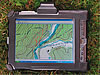 Figure 1
Our preferred method uses either a Trimble GeoXM pocket PC or an xPlore iX104C pre-loaded with bit-mapped scans of topographic maps and aerial photos of our field areas. These images are georectified and re-projected within ArcGIS and then downloaded to ArcPAD along with shapefiles (data files for spatial information). These files incorporate attribute data, such as lithology names, orientation measurements, and other pertinent outcrop data recorded on location (see Appendix A for examples [footnote 1]). Linear features, such as contacts and faults, are recorded in a separate shapefile by tracing or walking the features in the field. Polygons of lithologic units are drawn in ArcPAD while in the field, based on current working hypotheses. We still record data in a field book as a backup, because battery power (typically about eight hours) or GPS signals can be lost prematurely. Once back in the office, we upload the ArcPAD data and interpretations recorded in the field to ArcGIS. We follow the uploading process with a visual examination of the days field data, and correct any field data entered in an incorrect format. It is important to emphasize that faults, contacts, and unit polygons must be interpreted and drawn on the digital (ArcPAD) map while on location in the field. This is easily accomplished using the digital methods described here, though geologists unfamiliar with these techniques might find that it initially requires more time in the field. A significant advantage to digital fieldwork is the ability to easily assemble draft versions of field maps, which can be continually evaluated in the field. We strongly advocate this iterative method of field mapping, having developed and tested it over several years of field courses and field research projects (De Paor and Whitmeyer, 2009; Whitmeyer et al., 2009). Ultimately, the working field map becomes the final version, and the ArcGIS shapefiles are then ready for export to KML files for use in Google Earth or other virtual globes.
Virtual 3-D presentation of geologic data
Background
Perhaps the most significant recent advance for geologic map and cross-section interpretation is software that facilitates virtual 3-D display of geologic data. GIS software, such as ArcGIS, has long incorporated 3-D terrain construction (e.g., ArcGIS 3-D Analyst) that allows users to view and analyze GIS data in a virtual 3-D environment. However, achieving the full potential of computerized display and evaluation of geologic maps has been hampered by such issues as the cost and steep learning curve of GIS software—months to years can be required to build a working knowledge of the software tools. These issues have been largely alleviated by the advent of Web-based global digital elevation model (DEM) databases (Google Earth, NASA World Wind), which have put virtual 3-D terrains at the fingertips of the novice user. These software packages are freely available, with intuitive, easy-to-use interfaces that only require a computer with high-speed Internet access. Access in the field is also possible with a remote wireless receiver.
Virtual globes became available shortly after Al Gore proposed a “Digital Earth” Internet browser in 1998. The first serious digital globe application was unveiled by NASA in 2001 as World Wind, which was designed to display planetary data in the new format of a rotatable 3-D globe. This was closely followed by the development of Keyhole Markup Language (KML) by the startup Keyhole Corporation. Googles subsequent purchase of Keyhole led to the release of Google Earth in 2005. Google Earth incorporates KML as the open-source scripting language that allows users to customize the presentation of geospatial data within the virtual globe interface. At present, most major virtual globes (Google Earth, World Wind, and Microsofts Virtual Earth) use KML as their scripting language (Wilson et al., 2007; Wernecke, 2009). KML is primarily responsible for the versatility of Google Earth as an effective medium for interactive presentation of geospatial data. This is accentuated when combined with COLLADA, an XML-based scripting language incorporated within Googles SketchUp program that allows users to include 3-D models within Google Earth. This is the method we use to design cross sections and structural map symbols as 3-D models, which are exported to specific locations and orientations within Google Earth.
Google Earth as an Interactive Presentation Tool
Over the past several years, Google Earth has become popular as a presentation tool for geoscience data. The ease with which images of geologic maps and other two-dimensional (2-D) data can be draped over the 3-D terrain and ortho-imagery within Google Earth (as “ground overlays”) has led to a flurry of quickly-rendered visual applications (e.g., USGS, 2006). There is no denying the effectiveness of viewing and interpreting current and historical geologic maps draped over a DEM, and this method certainly provides a level of map evaluation unimaginable by previous generations of geoscientists. Unfortunately, in many cases, these images are imported as excessively large files (10 MB or larger), which can slow the performance of Google Earth dramatically. A much better solution is to subdivide maps into nested images of increasing resolution and create a pyramid structure in which each image resolution level appears at the appropriate altitude for viewing as the user zooms in or out (see De Paor and Whitmeyer, 2010,for details). This is the method virtual globes use to quickly and smoothly display aerial photography of increasing resolution as one zooms closer to the ground surface.
Ground overlays are an effective display and presentation tool, but they dont encourage much interaction or inquiry from the user. To achieve the full potential of virtual globes as an interactive, inquiry-driven resource, we have developed a methodology for the presentation of geologic maps within Google Earth that goes beyond traditional 2-D imagery. Principal components of these maps include
- Units and contacts as individually selectable objects that can be turned on and off;
- Floating orientation symbols that show strike and dip or trend and plunge in the proper 3-D orientation at the precise location where measured in the field;
- Field data, such as outcrop photos or biostratigraphic information, as clickable objects linked to their field locations;
- Map legends as screen overlays; and
- Cross sections as vertical models that can emerge from the ground surface at the appropriate positions.
BUILDING A GOOGLE EARTH INTERACTIVE GEOLOGIC MAP
Case Study: Digital Mapping in Western Ireland
Digital field mapping and data collection for our case studies was conducted in conjunction with the James Madison University (formerly Boston University) field course in western Ireland (Johnston et al., 2005; Whitmeyer et al.,2009). We chose field areas with well-known stratigraphic relationships and interesting, but not overly complex, structural relationships. The Knock Kilbride field area (Appendix C [see footnote 1]) consists of a sequence of early to middle Paleozoic, moderately to steeply dipping sedimentary units, with several cross-cutting normal faults that offset the stratigraphy (Graham et al., 1989; Chew et al., 2007). The Ben Levy field area (Appendix D [see footnote 1]) is located 10 km southeast of Knock Kilbride (Fig. 2) and features the same stratigraphic units, with the addition of overthrust Neoproterozoic schists (Williams and Harper, 1991). This field area is important in a regional sense, because the boundary between the Neoproterozoic schists and the Paleozoic sedimentary rocks has been interpreted as the suture between the exotic Connemara Terrane and the South Mayo Trough (Williams and Rice, 1989; Dewey and Ryan, 1990).
|
Simplified geologic map of central western Ireland showing the Knock Kilbride and Ben Levy field areas near the eastern contact of the South Mayo Trough and Connemara terranes (modified from Chew et al., 2007). |
 Figure 2
Over the past five years, large data sets were collected using the digital techniques described in the previous sections. By incrementally moving our field areas along the mountains of Knock Kilbride and Ben Levy each year, we assembled composite digital data sets of hundreds of points that blanketed our field areas (Fig. 3). The overwhelming majority of accurate data made occasional incorrect orientation measurements easy to identify. Anomalous points were reevaluated during subsequent field days and fixed if necessary. ArcGIS attribute tables and shapefiles were exported and converted to KML using a combination of ArcGIS, Arc2Earth™ software, and custom scripts. Although current versions of ArcGIS (9.3) and Google Earth Pro (5.0) facilitate the exchange of data between shapefiles and KML, efficient export of data from lengthy attribute tables remains a challenge. A template for doing this is included in Appendix A (see footnote 1).
|
Composite geologic map of the Knock Kilbride field area in ArcGIS, showing the accumulation of hundreds of data points from several summers of digital mapping. Points, lines, and polygons were exported from this ArcGIS map to create the Google Earth geologic map in Appendix C and shown in Figure 4. |
 Figure 3
Assembling Google Earth Map Components
One of the useful aspects of a Google Earth geologic map is the ability to view and evaluate geologic units as semitransparent, colored polygons superimposed on the 3-D terrain. However, in many regions, the stock Google Earth aerial imagery is too poorly resolved for professional geologic applications. To improve the Google Earth imagery for western Ireland, we created image pyramids from high-resolution aerial photos to serve as our base map. Individual photo tiles occupy only 20 KB and load efficiently, which avoids delays that occur when Google Earth loads multi-megabyte images. This technique is also applicable to environmental maps on which seasonal change needs to be presented, because Google Earth ground images are usually months, if not years, out of date.
Google Earth contains tools to create placemarks (points), polylines, and polygons, and one approach to generating geologic map components is to use these built-in tools. However, caution is required when using placemarks for geologic map symbols: Though placemarks are fixed to a specific location, the placemark icon always rotates to be perpendicular to the point of view of the user. This isnt a problem when marking unoriented outcrop data (e.g., identifying fossil locations), but it will not work for data with an associated spatial orientation, like strike and dip symbols or outcrop photographs taken in a referenced direction.
One approach to presenting strike and dip data is to generate images of strike and dip symbols with a transparent background (e.g., PNG or TIFF format) and use the “Image Overlay” feature to drape them in Google Earth (Fig. 4). This works only when viewed from above; from other viewpoints, symbols can be distorted by oblique projection onto a sloping terrain. Our preferred solution is to generate 3-D strike and dip symbols that hover a few meters above the ground in their proper latitude/longitude location and orientation (Fig. 5). This display method takes some familiarization, as most geoscientists are used to seeing orientation symbols on a flat map surface, but we find that these 3-D symbols are often easier for nongeologists to comprehend and thus preferable to traditional symbology.
|
Oblique, tilted view of the Knock Kilbride geologic map showing strike and dip symbols as colored ground overlays. Note how the orientation symbols get distorted in areas of high relief. |
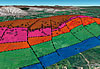 Figure 4
|
Tilted view (looking northwest) showing a vertical cross section extracted from the terrain surface of the Ben Levy geologic map. Note the colored, 3-D strike and dip symbols (both bedding and foliation) that hover a few meters off the terrain surface. |
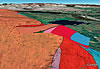 Figure 5
The latest version of KML includes a “photo overlay” feature. Unlike image overlays, photo overlays are automatically structured into image pyramids when imported into Google Earth; thus, very high-resolution images may be loaded without slowing system response. Appendix B (see footnote 1) is an example of a photo overlay created from an oriented field photograph of pillow lavas near the Knock Kilbride field area. The viewer can zoom in on the outcrop photo until fine detail is visible.
Generating 1-D and 2-D features, such as traces of contacts or faults, and surface exposures of stratigraphic units works reasonably well using the Google Earth polyline and polygon tools. However, draw levels cannot be specified for these features. This is a problem when map images need to be overlain in a specific order, as with our maps, on which imported aerial photographs must underlie stratigraphic units and symbology. Our approach is to create colored polygons for each stratigraphic unit in PNG format with a transparent background. These images are directly and easily exportable from an ArcGIS geologic map. After obtaining the latitude and longitude coordinates for the boundaries of each image exported from ArcGIS, we overlaid these images in the correct locations in Google Earth. Since image overlays can be assigned a specific draw level, we ensured that the images were stacked in the proper order for viewing. The advantage of overlaying each unit as a separate image is that users can toggle the display of each unit on or off in the Google Earth “places” window.
Geologic maps generally include a map legend or explanation. This is accomplished within Google Earth by using the “screen overlay” function. This function cannot be invoked directly from the pull-down menus in Google Earth, but requires KML coding using a text editor (see Appendix A for an example [footnote 1]). The position of the screen legend is fixed, but it can be toggled on and off to view the features on the Google Earth globe. Scale bars and north arrows are not included in screen legends, as the underlying globe can be zoomed, panned, and rotated independent of the fixed screen overlay.
Cross Sections
Since the initial work of Smith (1815), it has been customary for geologic maps to include vertical interpretations of the subsurface as cross sections. Unfortunately, many nonprofessionals and students find it difficult to visualize 3-D structures using traditional paper geologic maps with cross sections and locations indicated on the map via thin lines marked A–A′, B–B′, etc. (Piburn et al., 2002; Kastens and Ishikawa, 2006). Fortunately, Google Earth has the capacity to incorporate 3-D models as user-generated structures. These models can be designed using Google SketchUp, exported as Collada script in .dae files, and positioned within Google Earth using KML or the “import model” menu. This is the basic method for creating and positioning vertical cross sections within Google Earth (Fig. 5). A newly developed technique allows users to “pull” a geologic cross section up out of the Google Earth ground surface using a slider control. This approach intuitively conveys the concept that cross sections represent subsurface geology. Creating these emergent cross sections does require some advanced KML programming; see De Paor and Whitmeyer (2010) for details.
Other Digital Techniques
Several digital mapping technologies are not discussed here because they involve equipment that is not typically carried by a field geologist. These include LiDAR (McCaffrey et al., 2008) and GigaPan (e.g., Schott, 2008), both of which require specialty equipment mounted on tripods. Further miniaturization and commercialization may lead to their general adoption by field geologists in the future.
CONCLUSIONS AND IMPLICATIONS
There are disadvantages to the digital mapping and geologic map presentation methods discussed in this paper. First is the initial time commitment needed to get comfortable with the hardware and software necessary for digital mapping. Some field workers may be reluctant to depend on computer equipment for collecting data in the field, and the necessity for keeping a hard copy backup of digital field data may induce some to wonder “why go digital?” in the first place. However, the ability to compile hundreds of measurements from many sources makes the benefits of digital data-gathering abundantly clear. In addition, since all modern professional geologic maps are published using computer-based graphics design programs, such as Adobe Illustrator or ArcGIS, field mappers can simplify and streamline the process by using coordinated computer equipment and software for the whole procedure of field data collection, interpretation, and map generation. Many academic and industry geoscientists have already reached this conclusion, such that a working knowledge of ArcGIS and digital field methods is no longer a luxury, but rather a necessary skill in todays selective, but lucrative, geoscience-related fields (AGI, 2009).
A limitation to interactive geologic maps rendered on virtual globes is their current inability to be repackaged for export as paper maps. Similar to civil engineers who need blueprints for the job site, geoscientists still have a need for paper geologic maps in situations where computer equipment is not readily available. This is one reason we prepare versions of final geologic maps in ArcGIS, which can be printed as traditional paper maps if desired. ESRI has developed virtual 3-D viewers (ArcGIS Explorer, ArcGlobe) that can use the same shapefiles and attribute tables that are incorporated into ArcGIS-generated paper maps. Ease of use is still an issue with these ESRI products, but their efficient data transfer between paper and virtual formats may prove to be an advantage over other virtual globes.
Developing interactive geologic maps for virtual globes requires new skills, such as KML scripting, but many of todays generation of technologically savvy students and professionals are quite comfortable with these new techniques. Computer-aided 3-D design (CAD) has long been standard in manufacturing and engineering industries. Plus, many of our students have grown up playing computer games with realistic, high-resolution images and view paper-based geologic maps and cross sections as antiquated. Perhaps the most important reason to develop interactive Google Earth–based geologic maps is their utility in presenting geologic data and interpretations in a format that is easier for the layperson or introductory-level student to understand. Individual geologic units can be directly related to the surface topography using transparent, selectable ground overlays. Important field data and photos of key features can be viewed and highlighted by tags that link to the precise location of an outcrop. Orientation symbols can be correctly oriented in 3-D space, making the concepts of strike and dip easier to grasp. Finally, cross sections, as interpretations of subsurface geology, are far more intuitive when the user can “pull” these vertical slices up out of the ground in their correct positions. Complete Google Earth geologic maps for our case study field areas in western Ireland are discussed in Appendix A and included as KMZ files in Appendix C (Knock Kilbride field area) and Appendix D (Ben Levy field area) (see footnote 1). Readers are encouraged to experiment with these interactive geologic maps to explore the methods discussed herein.
ACKNOWLEDGMENTS
The authors thank Chris Condit, Lisel Currie, and Stephen Johnston for helpful reviews and students and faculty from the James Madison University (JMU) Field Course in Ireland for digital mapping assistance. This work was funded in part by National Science Foundation grants EAR-0711092 and DUE-0837049, and by the JMU College of Science and Mathematics.
REFERENCES CITED
- American Geological Institute (AGI), 2009, Status of the Geoscience Workforce 2009: http://www.agiweb.org/workforce/reports/2009-StatusReportSummary.pdf (last accessed 27 Jan. 2010).
- Chew, D.M., Graham, J.R., and Whithouse, M.J., 2007, U-Pb zircon geochronology of plagiogranites from the Lough Nafooey (= Midland Valley) arc in western Ireland: Constraints on the onset of the Grampian orogeny: Journal of the Geological Society, v. 164, p. 747–750.
- Condit, C.D., 1995, DDM.SVF: A prototype Dynamic Digital Map of the Springerville volcanic field, Arizona: GSA Today, v. 5, no. 4, p. 69, 87–88.
- Cuvier, G., and Brongniart, A., 1908, Essai sur la Géographie Minéralogique des Environs de Paris, avec une Carte Géognostique, et des Coupes de Terrain: Paris, Baudouin, 278 p.
- De Paor, D.G., and Whitmeyer, S.J., 2009, Innovations and obsolescence in geoscience field courses: Past experiences and proposals for the future, in Whitmeyer, S.J., Mogk, D.W., and Pyle, E.J., eds., Field Geology Education: Historical Perspectives and Modern Approaches: Geological Society of America Special Paper 461, p. 45–56.
- De Paor, D.G., and Whitmeyer, S.J., 2010, Geological and geophysical modeling using data pyramids and virtual globes: Computers and Geosciences, in press.
- Dewey, J.F., and Ryan, P.D., 1990, The Ordovician evolution of the South Mayo trough, western Ireland: Tectonics, v. 9, p. 887–903.
- Gore, Al, 1998, The Digital Earth: Understanding our planet in the 21st Century: Los Angeles, California, California Science Center, 31 Jan. 1998, The Fifth International Symposium on Digital Earth, http://www.isde5.org/al_gore_speech.htm (last accessed 26 Jan. 2010).
- Graham, J.R., Leake, B.E., and Ryan, P.D., 1989, The geology of South Mayo, western Ireland: Edinburgh, Scottish Academic Press, 75 p.
- Griffith, R.J., 1838, Outline of the geology of Ireland: Dublin, Railway Commissioners.
- Hitchcock, C.H., 1878, The Geology of New Hampshire: Concord, New Hampshire, 3 volumes, 2061 p.
- Johnston, S., Whitmeyer, S.J., and De Paor, D., 2005, New developments in digital mapping and visualization as part of a capstone field geology course: Geological Society of America Abstracts with Programs, v. 37, no. 7, p. 145.
- Kastens, K.A., and Ishikawa, T., 2006, Spatial thinking in the geosciences and cognitive sciences: A cross-disciplinary look at the intersection of the two fields, in Manduca, C.A., and Mogk, D.W., eds., Earth and Mind: How Geologists Think and Learn about the Earth: Geological Society of America Special Paper 413, p. 53–76.
- Knoop, P.A., and van der Pluijm, B., 2006, GeoPad: Tablet PC-enabled field science education, in Berque, D., Prey, J., and Reed, R., eds., The Impact of Pen-based Technology of Education: Vignettes, Evaluations, and Future Directions: West Lafayette, Indiana, Purdue University Press, p. 103–114.
- Kramer, J.H., 2000, Digital mapping systems for field data, in Soller, D.R., ed., Digital Mapping Techniques’00—Workshop Proceedings: U.S. Geological Survey Open-File Report 00-325, p. 13–19.
- Longley, P.A., Goodchild, M., Maguire, D.J., Rhind, D.W., and Lobley, J., 2001, Geographic Information Systems and Science: Hoboken, New Jersey, John Wiley & Sons, 454 p.
- McCaffrey, K.J.W., Jones, R.R., Holdsworth, R.E., Wilson, R.W., Clegg, P., Imber, J., Holliman, N., and Trinks, I., 2005, Unlocking the spatial dimension—Digital technologies and the future of geoscience fieldwork: Journal of the Geological Society, v. 162, p. 927–938.
- McCaffrey, K.J.W., Feely, M., Hennessy, R., and Thompson, J., 2008, Visualization of Folding in Marble Outcrops, Connemara, western Ireland: An application of virtual outcrop technology: Geosphere, v. 4, p. 588–599.
- Mies, J.W., 1996, Automated digital compilation of structural symbols: Journal of Geoscience Education, v. 44, p. 539–548.
- Piburn, M.D., Reynolds, S.J., Leedy, D.E., McAuliffe, C.M., Burk, J.P., and Johnson, J.K., 2002, The Hidden Earth: Visualization of Geologic Features and their Subsurface Geometry: National Association for Research in Science Teaching, p. 1–48.
- Ray, P.T.C., 2002, GIS in Geoscience: The recent trends: The Geospatial Resource Portal, GISdevelopment.net, http://www.gisdevelopment.net/application/geology/mineral/geom0012.htm (last accessed 25 Jan. 2010).
- Schetselaar, E., 1995, Computerized field-data capture and GIS analysis for generation of cross sections in 3-D perspective views: Computers and Geosciences, v. 21, p. 687–701.
- Schott, R., 2008, GigaPanner, Exploring the Creation and Uses of GigaPixel Images with a Focus on the GigaPan Project: http://www.gigapanner.com/ (last accessed 27 Jan. 2010).
- Selner, G.I., and Taylor, R.B., 1993, GSMAP and other programs for the IBM PC and compatible microcomputers, to assist workers in the earth sciences (version 9): U.S. Geological Survey Open-File Report 93-511, 363 p.
- Smith, W., 1815, A geological map of England and Wales and part of Scotland: London, British Geological Survey, 1 sheet.
- USGS, 2006, San Francisco Bay Region Geology and Geologic Hazards, Geologic Downloads: U.S. Geological Survey, http://geomaps.wr.usgs.gov/sfgeo/geologic/downloads.html (last accessed 26 Jan. 2010).
- Wernecke, J., 2009, The KML Handbook: Geographic Visualization for the Web: Upper Saddle River, New Jersey, Addison-Wesley, 368 p.
- White House Office of Science and Technology Policy (OSTP), 2000, Statement by the president regarding the United States decision to stop degrading global positioning system accuracy: Washington, D.C., The White House, http://clinton3.nara.gov/WH/EOP/OSTP/html/0053_2.html (last accessed 22 Jan. 2010).
- Whitmeyer, S.J., Feely, M., De Paor, D.G., Hennessy, R., Whitmeyer, S., Nicoletti, J., Santangelo, B., Daniels, J., and Rivera, M., 2009, Visualization techniques in field geology education: A case study from Western Ireland, in Whitmeyer, S.J., Mogk, D.W., and Pyle, E.J., eds., Field Geology Education: Historical Perspectives and Modern Approaches: Geological Society of America Special Paper 461, p. 105–115.
- Williams, D.M., and Harper, D.A.T., 1991, End-Silurian modifications of Ordovician terranes in western Ireland: Journal of the Geological Society, v. 148, p. 165–171.
- Williams, D.M., and Rice, A.H.N., 1989, Low-angle extensional faulting and the emplacement of the Connemara Dalradian, Ireland: Tectonics, v. 8, p. 417–428.
- Wilson, T., Burggraf, D., Lake, R., Patch, S., McClendon, B., Jones, M., Ashbridge, M., Hagemark, B., Wernecke, J., and Reed, C., 2007, KML 2.2—An OGC Best Practice: Open Geospatial Consortium, Document OGC 07-113r1, http://portal.opengeospatial.org/files/?artifact_id=23689 (last accessed 27 Jan. 2010).