
Full Text View
GSA Today
![]()
Article, pp. 4-11 | Abstract | PDF (336KB)
Virtual Rocks
| Table of Contents |
|---|
|
Search GoogleScholar for
Search GSA Today |
Abstract
Three-dimensional digital models of geological objects are relatively easy to create and geolocate on virtual globes such as Google Earth and Cesium. Emerging technologies allow the design of realistic virtual rocks with free or inexpensive software, relatively inexpensive 3D scanners and printers, and smartphone cameras linked to point-cloud computing services. There are opportunities for enhanced online courses, remote supervision of fieldwork, remote research collaboration, and citizen-science projects, and there are implications for archiving, peer-review, and inclusive access to specimens from inaccessible sites. Virtual rocks can be gradually altered to illustrate geological processes such as weathering, deformation, and metamorphic mineral growth. This paper surveys applications in a wide range of geoscience subdisciplines and includes downloadable examples. Detailed instructions are provided in the GSA Supplemental Data Repository1.
Manuscript received 29 June 2015; accepted 7 March 2016
doi: 10.1130/GSATG257A.1
1 GSA Supplemental Data Repository Item 2016173, detailing techniques for creating virtual specimens along with figure animations, is online. If you have questions, please contact GSA Today, P.O. Box 9140, Boulder, CO 80301-9140, USA; gsatoday@geosociety.org.
Introduction
In recent decades, numerous virtual field trips have been created to simulate in-person field excursions; however, one aspect of physical fieldwork is not commonly replicated: virtual explorers do not often return to their computer desktops with collections of virtual rocks! There are multiple justifications for creating interactive 3D digital models of rocks, minerals, fossils, drill core, geo-archaeological objects, and outcrops. For example, one can (i) reveal 3D features hidden inside solid specimens; (ii) archive samples destined for destructive testing; (iii) prepare for field trips and reinforce learning and retention after the fact; (iv) aid peer-review and supplement electronic publications; (v) give access to geological materials for disabled and other non-traditional students; and (vi) provide access to collections locked away in storage drawers, given that museums and other repositories display only a small fraction of their holdings.
The concept of a virtual specimen is not new. Following the mechanical tomography of Sollas (1904), Tipper (1976) used a grinding wheel to serial-section fossils. He traced outlines with a digitizing tablet, created 3D models with a mainframe computer, and interacted with them using a graphics storage tube (relatively youthful readers can image-google “graphics storage tube”), exploring previously hidden inner surfaces.
Virtual geological collections already exist online, and readers may simply link content to their own virtual field trips, online courses, and social media pages. Reynolds et al. (2002) and Bennington and Merguerian (2003) used QuickTime Virtual Reality (QTVR) to display interactive digital specimens. The Smithsonian Museum has a large collection of scanned 3D objects (Smithsonian, 2016), and the British Geological Survey (2016) has assembled more than 1,800 virtual fossils. Numerous LiDAR models of outcrops have been made (Clegg et al., 2005; McCaffrey et al., 2008; Buckley et al., 2010; see also Passchier, 2011, and VOG, 2016).
More recently, geoscientists have created many virtual specimens for paleontological functional analysis, digital exchange of research data, and teaching in a range of geoscience subdisciplines. For example, Pugliese and Petford (2001) revealed 3D melt topology of veined micro-diorite, and Bates et al. (2009) estimated dinosaur bone mass from models.
Modelers have long used 3D scanners, and, more recently, 3D printers (Hasiuk, 2014) to create ever-more sophisticated virtual objects. Cohen et al. (2010) reconstructed archaeological vessels from virtual ceramic shards, harnessing the computer’s power to solve 3D jigsaw puzzles. Engineering geologists Dentale et al. (2012) used FLOW-3D® software to test a virtual breakwater built out of individual virtual stones and accropodes™. Medical CT-scanning methodologies were used by Hoffmann et al. (2014) to study buoyancy in virtual cephalopods, by Carlson et al. (2000) for igneous texture studies, and by Pamukcu et al. (2013) to examine glass inclusions in quartz crystals. Rohrback-Schiavone and Bentley (2015) employed GIGAmacro™ hardware to create grain-scale sedimentological models. Root et al. (2015) compared models of Neolithic monuments in Ireland and the Middle East, while Mounier and Lahr (2016) created a 3D model of the skull of the common ancestor of humans and Neanderthals. Structural geologists Thiele et al. (2015) gained new insights into en échelon vein formation, and Favalli et al. (2012) modeled outcrops, a volcanic bomb, and a stalagmite. They concluded that the quality of virtual outcrops or specimens is comparable to LiDAR outcrops or laser-scanned specimens, respectively.
In recent years, the most exciting developments in 3D modeling include the availability of smartphone apps and associated point-cloud computing services that non-specialists can quickly master. The purpose of this paper is to highlight the recent, current, and potential future role of virtual specimens in diverse aspects of geoscience education and research.
Creating Virtual Specimens with SketchUp
Virtual specimens can be created with a digital camera and SketchUp (2016). SketchUp exports a model as a COLLADA file optionally zipped with a KML document and one or more texture images in a KMZ archive. COLLADA (Arnaud and Barnes, 2006) is the format used to display 3D buildings, bridges, etc., on the Google Earth terrain, but De Paor and Piñan-Llamas (2006) and De Paor and Williams (2006) discovered that they could create much larger crustal models that can be made to emerge from the subsurface (De Paor, 2007) with a slider control (see also Chen et al., 2008; De Paor and Whitmeyer, 2011; Blenkinsop, 2012; Boggs et al., 2012; Karabinos, 2013; St. John, 2014).
Slab-Shaped COLLADA Models
Consider a rock, which we here define as the verilith (Latin for “real rock”) with two parallel sides and minor thickness, such as slate, shale, flagstone, or any hand specimen sliced thinly by a rock saw. Figure 1 shows a sample collected from a limestone quarry near Rheems, Pennsylvania, USA (De Paor et al., 1991; De Paor, 2009). Photographs of the flat sides were applied to a rectangular block in SketchUp (Fig. 1 inset) following the method of De Paor and Piñan-Llamas (2006; see also De Paor, 2007), and the later rediscovery of the method by Van Noten (2016). Model construction is explained in detail in the GSA Supplemental Data Repository (see footnote 1), but the process can be summarized as the digital equivalent of gluing photographs to plywood and cutting object outlines with a jigsaw. The Rheems model was exported to Google Earth and placed at its collection site. A KML file was scripted to make the specimen rotate about a vertical axis in response to the Google Earth slider. (The COLLADA models in the online versions of all figures respond to mouse drags or touch swipes—see the GSA Supplemental Data Repository [footnote 1]). In lab class, students can clearly see that the limestone bridges crossing calcite veins are not identical in shape on either side of the specimen, and they are challenged to visualize the complex 3D forms in the specimen’s interior, which was the purpose of the exercise in this case.
|
Virtual rock created with SketchUp and geolocated at collection site, Rheems Quarry, Pennsylvania, USA. Online version can be rotated, and is available at dx.doi.org/10.1130/GSATG257.S1. ©2016 Google Inc. Image: Landsat. Inset: Photographing hand specimen at arm’s length. Background is irrelevant as it will be cropped. |
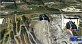 Figure 1
Ovoid- and Hemi-Cylinder–Shaped COLLADA Models
A similar approach was taken with ellipsoidal, or ovoid, and hemi-cylindrical specimens, as illustrated by KMZ downloads accompanying this paper. Six photographs were draped over a model of an ovoidal beach pebble in the ± x, ± y, and ± z directions. To represent cut drill core, cylinders were extruded from circles in SketchUp, then sliced longitudinally, with core photographs applied as textures. When imported into Google Earth, such specimens can be made to rise out of the subsurface at their drill site in response to the slider control. This was done as a proof-of-concept by De Paor (2007) and implemented on a large scale using Big Data IODP repositories by St. John (2014).
Complex Specimens and 3D Scanners
It is possible to create complex models with SketchUp, but for intricate specimen shapes, 3D scanning is less tedious. A relatively inexpensive NextEngine (2016) scanner was used to model pseudotachylite from Vredefort, South Africa—Earth’s oldest and largest known impact structure (De Paor et al., 2010; Fig. 2). Rock specimens had been collected during legacy graduate student mapping by Simpson (1978) before the region became a protected World Heritage Site. Specimens were retrieved from long-term storage and scanned. Open-source software (MeshLab, 2016) (zBrush is a sophisticated, albeit expensive alternative [Michael, 2016; TurboSquid, 2016]) was used to clean scanning errors and reduce model size. Google Earth literally shreds models with more than 64,000 vertices, so reducing the number of vertices is essential for most raw scans. Of the many vertex reduction options in MeshLab, the only one that worked whilst maintaining specimen quality was Quadric Edge Collapse Decimation (see the GSA Supplemental Data Repository [footnote 1]). The model was exported from MeshLab in COLLADA format for use with Google Earth.
|
Pseudotachylite specimen from Vredefort impact structure. ©2016 Google Inc. Image: Landsat. Map by Hartwig Frimmel. Online version can be rotated, and is available at dx.doi.org/10.1130/GSATG257.S2. |
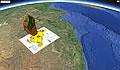 Figure 2
Multi-View Stereo and Structure from Motion
The most exciting recent modeling innovations are in the field of multi-view stereo (MVS) photogrammetry. Se and Jasiobedzki (2008) used video imagery from an unmanned vehicle and the Simultaneous Localization and Mapping (SLAM) algorithm to monitor an active mine. An algorithm called Structure from Motion (SfM) uses multiple still images from a smartphone or other digital camera to build 3D models. Snavely et al. (2008) and Enqvist et al. (2011) developed non-sequential SfM, enabling model construction from image searches (Schonberger et al., 2015). However, Sakai et al. (2011) require only two photographs, and Gilardi et al. (2014) created 3D beach pebbles from a single orthogonal photograph.
The bleeding edge of SfM technology is Autodesk® Memento (2016), which at the time of this writing was in public beta-test phase. It was slated for commercial release in May 2016 under the new name Autodesk® ReMake. It promises to accommodate billions of vertices with no limit on the number or resolution of images. Such models will doubtless be too large to embed directly into Google Earth or Cesium virtual globes unless they evolve in tandem, but will be accessible from virtual field trip stops via HTML hyperlinks to modern browsers (Gemmell, 2015), of which the fastest appears to be Waterfox (2016).
VisualSFM (Wu, 2013) is an open-source application with enhanced SfM editing capabilities; however, it requires command-line competency and is not for the faint-of-heart. PhotoScan from Agisoft (2016) is a more popular choice (Pitts et al., 2014; Shackleton, 2015) and whilst not free, is deeply discounted for education. Bemis et al. (2014) review other SfM methodologies, including UAV outcrop mapping. Probably the easiest SfM application for beginners, however, is Autodesk’s 123D Catch.
Schott (2012) modeled mud cracks using Autodesk’s original SfM application, PhotoFly—since renamed 123D Catch—which is freely available from Autodesk (2016; there is a premium version with a US$10 monthly fee). Karabinos (2013) used it to create outcrop and boulder models. De Paor (2013) described the process of porting 123D Catch models to Google Earth by processing them through MeshLab. Bourke (2015) used SfM to model an indigenous Australian rock shelter; Lucieer et al. (2013) mapped landslide displacement using SfM and UAV photography; and MCG3D (2015) made particularly good use of annotation capabilities in a geo-tourism application.
Figure 3 shows a mantle xenolith from Salt Lake (Āliamanu) Crater, adjacent to Pearl Harbor, Hawaii. The verilith was collected by Michael Bizimis, University of South Carolina, and mailed to the author for SfM modeling. Because the most important part of this specimen is the saw-cut surface, it was possible to reduce the 4 MB raw scan down to less than half a MB without losing any resolution on the cut surface. Peridotite mineralogy is easily identified by most students in the final model despite its modest resolution.
|
Structure from Motion model of a mantle xenolith from Salt Lake (Āliamanu) Crater, Hawaii. Caldera marked in red. Verilith provided by Mike Bizimis. ©2015 Google Inc. Online version can be rotated, and is available at dx.doi.org/10.1130/GSATG257.S4. |
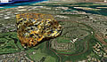 Figure 3
The downloads include a KMZ model of Acasta Gneiss, the oldest whole rock ever dated, at 4.03 Ga. Its verilith was loaned by Sam Bowring, MIT, and the model created with 123D Catch can be viewed in the source location in Northwest Territories by thousands of people who will never go there in person. Instructors can use these and other models that are shared by colleagues in SketchUp’s 3D Warehouse (2016), the 123D Catch Gallery (2016), SketchFab (2016), Thingiverse (2016), and other digital repositories. For example, the author downloaded fossil models from Brain (2016), processed them in MeshLab, and geolocated them in Google Earth. Figure 4 shows a virtual ammonite from Semington, Wiltshire, England, and the downloads include a model of Gryphaea arcuate from Hock Cliff, England.
|
Ammonite from Semington, Wiltshire, England. ©2010 Google Inc. Image GetMapping plc. Online version can be rotated, and is available at dx.doi.org/10.1130/GSATG257.S5. |
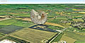 Figure 4
Sometimes, people may want to display interactive specimens not linked to a particular location—for example, when the location is not known. There are three approaches: First, COLLADA models can be viewed with software such as Adobe PhotoShop™ or Apple Preview™. Second, Google Earth version 6.0 (or earlier) can be downloaded from a legacy software portal such as FileHippo (2016). In early versions of Google Earth, the Primary Database could be selected and made transparent with a slider, hiding the surface imagery. The accompanying KMZ downloads include a rotatable, zoomable apatite crystal in Google Earth v. 6.0. The third approach is to embed a COLLADA model directly in a web page as in the case of the halite crystal lattice in the GSA Today cover image(seedx.doi.org/10.1130/GSATG257.S3 for interactive online version). This is the best option for viewing on mobile devices. By rota ting lattice models with a touchscreen swipe, students can see non-intuitive symmetry elements, such as a cubic crystal’s three-fold axes, and the background image adds context. The process of displaying interactive COLLADA models in HTML 5 is far from self-evident, but this paper’s sample file, using a 3D library from GitHub (2016), can be downloaded and modified. Readers can simply search for “files/halite.dae,” and replace that URL with another file of their choice.
Viewing Virtual Specimens in Web Browsers
Manipulating virtual rocks using the Google Earth desktop application is tedious due to the limitations of KML, an XML-based scripting language that has changed little in a decade and lacks basic programming features such as do-loops. Google Earth was available as a more versatile web browser plugin and application program interface (API), but that has been deprecated effective December 2015. A plugin-free API is expected in the not-too-distant future; meanwhile, an alternative approach is to convert models for viewing on the web-based Cesium virtual globe (Cozzi and Ring, 2011) using the glTF file format. A glTF version of the Vredefort specimen may be viewed at GEODE (2016) using the Chrome web browser (Chrome is the only browser that currently handles models in Cesium flawlessly). See the GSA Supplemental Data Repository (footnote 1) for technical details. Viewing in a web browser has distinct advantages because models can be manipulated with several JavaScript controls, such as radio buttons, numeric text fields, and multiple horizontal and vertical sliders. A web-based virtual globe hides irrelevant menu options that could be distracting to wanderlust-prone students and is accessible via mobile devices. Web-based presentation is important for building large searchable databases of virtual specimens in the future. Because HTML, KML, COLLADA, and glTF files are human-readable (not binary computer code), tags in multiple languages can be added for search purposes.
Changing Virtual Rocks with Time
Many undergraduate students have great difficulty understanding length and time scales of rock formation and change (Kortz and Murray, 2009). Virtual rocks can potentially help them visualize changes such as weathering, deformation, and metamorphism. For example, the KMZ downloads include a Google Earth view of New England with an emergent crustal block that is raised 20 km revealing the depth of garnet grade metamorphism. Students can zoom into the block’s base and find a virtual rock in which virtual garnet crystals grow with time. The speed of the simulation can be controlled using the Google Earth time slider. Ultra-slow animations spanning a three-hour lab or a three-month course, during which a specimen’s location, shape, or appearance is gradually modified, may help convey geological scales of space and time. This offers the possibility of viewing models of weathering, deformation, metamorphism, etc., in what may feel to students like geological time, because it is so slow compared to the pace of their digital lifestyles.
Discussion
Computer-generated 3D models of rocks cannot fully replace their veriliths, but they can significantly enhance online geoscience education and extend the range of rocks to which both onsite and distance education students are exposed. If online classes are to compete with onsite, we need to give students control over manipulable virtual specimens. Students engaged in physical fieldwork can also benefit, for example, by creating and uploading models for their instructors or peers to help identify. Smartphone technology opens up the possibility of data collection by non-professional citizen scientists. Crowd-sourcing in geoscience (Whitmeyer and De Paor, 2014) has been limited by the need for advanced skills, however, citizens can create 3D models and share them with remote experts. In Project Mosul (2016), archaeologists virtually rebuilt artifacts destroyed by ISIS militants using crowd-sourced tourist photographs. That project has extended to include virtual reconstruction of Katmandu’s cultural sites following the 2015 earthquake. Geoscientists with access to vulnerable sites can build image collections in advance of potential destructive events such as earthquakes, fires, floods, etc. (e.g., Ure, 2015). Instructors can ask every student in a class to take a cellphone photo of a specimen or outcrop from a variety of angles and build a model to which all students feel they have contributed.
Another justification for virtual rocks is their potential use in peer review of manuscripts whose analyses and conclusions depend critically on the correct identification of specimens. Reviewers currently rely on authors to interpret rocks. In future, they could ask to see 3D models—a more realistic request than having rocks mailed to them overland. Authors could embed virtual specimens in 3D PDF or HTML5 files as supplementary documents accompanying publications. As one anonymous reviewer of this paper wrote,
“I would not be surprised if in future, journals required 3D representations of outcrops and samples used within their publications. The ability to tag these with locations in a publicly available dataset could revolutionize structural geology and tectonics research. Imagine investigating a new field area and being able to download samples collected there by previous workers alongside their papers. This could reduce a lot of wheel reinventing!”
Not all rocks are suitable for modeling. The holes in scoriaceous basalt are particularly difficult to handle. Even with photogenic specimens, it may be advisable to wait for overcast conditions in order to avoid deep shadows that will not correspond to the sun’s direction in later viewings. If very high resolution is required, and rotation of the viewpoint is not essential, then GIGAmacro scans may be preferable to a 3D model (Bentley, 2015). Some models have gaps in the wireframe where they were in contact with a table or scanner turntable. These can be covered with a plain gray surface in MeshLab, otherwise students may be confused by the view into the interior of the specimen. As with art and sculpture restoration, a plain gray patch is preferable to artistic interpretation of the missing material. If a model does not truly reflect a verilith, that fact should be clearly stated. NextEngine distorts the rock texture into tiger stripes at the turntable contact as seen in the Vredefort specimen. If not cleaned up, these artifacts need to be pointed out to students.
Conclusions
Every (physical) surfer knows that the key to success is to not be too far ahead nor too far behind the currently breaking wave. It is too soon to tell whether COLLADA models on Google Earth will give way to glTF models on Cesium, or to the next unknown wave. File formats such as .doc and .pdf persist for decades. Others such as .wpd fade away. Currently, the most sharable 3D model formats include .dae and .obj, but this may quickly change.
Examination of rocks in the field remains important—indeed vital—but field geologists face many restrictions. For the author, this has included encounters with armed security guards in Spain, an angry muskox on Ellesmere Island, truculent farmers in western Ireland, and liability-averse coastal homeowners in New England. In many locations, collecting specimens may be difficult, dangerous, prohibited, or environmentally unfriendly. Interactive virtual specimens offer a partial solution to access issues for disabled and non-traditional students as legacy specimens collected in less restrictive times can be taken out of storage and brought back to life. After examining physical specimens in lab class, students can be given access to 3D scans for study time.
Virtual rocks can be combined with other visualizations to fill a gap in the size range between LiDAR outcrops and microscopic visualizations such as virtual thin sections. The terrain represented on virtual globes is rarely resolved even to outcrop scale, so there is a need for background auxiliary visualizations to give hand specimens a geographical context. Common examples include Google Street View, Photo Spheres, and GigaPans (e.g., Dordevic et al., 2015). Richards (2011) pioneered the concept of an “Easter-egg-hunt.” Students are presented with digital images such as small-scale cross-bedding samples and are challenged to zoom in on the outcrop location from which the specimen was collected by studying a GigaPan. Bentley (2015) used a comparative GigaPan viewer to combined a GigaPan of the Massanutten Sandstone with an instructor’s tracing of fossil tracks. Gessner et al. (2009) studied rock fractures using digital photogrammetry, and Sørensen et al. (2015) demonstrated that point-cloud models of outcrops photographed at 40 m were competitive with LiDAR scans. Outcrop-scale models can benefit from cut-aways following the design principles in Lidal et al. (2012).
Inexpensive Virtual Reality (VR) and Augmented Reality (AR) software and hardware such as FreshAiR, Poppy3D, and Google Cardboard round off an effective, immersive, virtual field trip experience (Cherney, 2015; Crompton and De Paor, 2015). Future possibilities include the use of 3D printers to create tactile models for blind students (Doyle et al., 2016). They could include audio tracks that respond to the model’s orientation in a blind student’s hands via embedded fiducials.
From the range of applications and future possibilities cited in this paper, it seems likely that members of every division of GSA could benefit from creating and sharing virtual specimens. They can even add an element of Dionysian entertainment to our Apollonian geoscience studies (Kingsbury and Jones, 2009; Petchkovsky, 2012). In conclusion, it is hard to deny the fact that “virtual rocks rock!”
Acknowledgments
This manuscript benefitted from comments by editor Jerry Dickens, reviewer John Geissman, and two anonymous reviewers. Melissa Beebe, Jessi Strand, Melissa Bates, Ernestine Brown, and Nathan Rogers assisted with scanning. This work was supported by the National Science Foundation under grants DUE-1323419 and DUE-1540652.
Supplementary Materials
This paper is supported by a Supplemental Data Repository item (see footnote 1) detailing techniques for creating virtual specimens. There are also KMZ samples that can be downloaded and opened with the Google Earth desktop application, a sample HTML file with an embedded interactive COLLADA model, and a sample 3D PDF contributed by Dr. Alan Pitts.
References Cited
- 123D Catch Gallery, 2016: http://123dapp.com/Gallery (last accessed 1 May 2016).
- 3D Warehouse, 2016: http://3dwarehouse.sketchup.com (last accessed 1 May 2016).
- Agisoft, 2016, Agisoft PhotoScan: http://www.agisoft.com and http://www.ausgeol.org/visualisations/ (last accessed 1 May 2016).
- Arnaud, R., and Barnes, M.C., 2006, COLLADA: Sailing the gulf of 3D digital content creation: Massachusetts, A.K. Peters Ltd., 237 p.
- Autodesk, 2016, 123D Catch: http://www.123dapp.com/catch (last accessed 1 May 2016).
- Bates, K.T., Manning, P.L., Hodgetts, D., and Sellers, W.I., 2009, Estimating the mass properties of dinosaurs using laser imaging and 3D computer modeling: PLoS One, v. 4, no. 2, e4532, doi: 10.1371/journal.pone.0004532.
- Bemis, S.P., Micklethwaite, S., Turner, D., James, M.R., Akciz, S., Thiele, S.T., and Bangash, H.A., 2014, Ground-based and UAV-based photogrammetry: A multi-scale, high-resolution mapping tool for structural geology and paleoseismology: Journal of Structural Geology, v. 69, p. 163–178, doi: 10.1016/j.jsg.2014.10.007.
- Bennington, J.B., and Merguerian, C.M., 2003, QuickTime virtual reality (QTVR): A wondrous tool for presenting field trips, specimens, and microscopy in traditional and web-based instruction: http://people.hofstra.edu/J_B_Bennington/qtvr/qtvr_object.html (last accessed 1 May 2016).
- Bentley, C., 2015, Four new GIGAmacro images of sedimentary rocks: AGU Blogosphere, http://blogs.agu.org/mountainbeltway/2015/12/23/four-new-gigamacro-images-of-sedimentary-rocks/ (last accessed 1 May 2016).
- Blenkinsop, T.G., 2012, Visualizing structural geology: From Excel to Google Earth: Computers & Geosciences, v. 45, p. 52–56, doi: 10.1016/j.cageo.2012.03.007.
- Boggs, K.J.E, Dordevic, M.M., and Shipley, S.T., 2012, Google Earth models with COLLADA and WxAzygy transparent interface: An example from Grotto Creek, Front Ranges, Canadian Cordillera: Geoscience Canada, v. 39, no. 2, p. 56–66, https://journals.lib.unb.ca/index.php/GC/article/view/19960/21886 (last accessed 12 May 2016).
- Bourke, P., 2015, Weld range rock shelter, Western Australia: https://skfb.ly/DXPO (last accessed 1 May 2016)
- Brain, A., 2016, Ammonite 1: http://www.123dapp.com/MyCorner/AdrianBrain-20378945/models (last accessed 1 May 2016).
- British Geological Survey, 2016, GB3D type fossils online project: http://www.3d-fossils.ac.uk/home.html (last accessed 1 May 2016).
- Buckley, S.J., Enge, H.D., Carlsson, C., and Howell, J.A., 2010, Terrestrial laser scanning for use in virtual outcrop geology: The Photogrammetric Record, v. 25, no. 131, p. 225–239, doi: 10.1111/j.1477-9730.2010.00585.x.
- Carlson, W.D., Denison, C., and Ketcham, R.A., 2000, High-resolution X-ray computed tomography as a tool for visualization and quantitative analysis of igneous textures in three dimensions: Visual Geosciences, v. 4, no. 3, p. 1–14, https://youtu.be/lqP9NJCLCUg (last accessed 1 May 2016).
- Chen, A., Leptoukh, G., Kempler, S., Nadeau, D., Zhang, X., and Di, L., 2008, Augmenting the research value of geospatial data using Google Earth, in De Paor, D., ed., Google Earth Science: Journal of the Virtual Explorer, v. 30, Paper 4, http://www.virtualexplorer.com.au/article/geospatial-data-using-google-earth (last accessed 16 May 2016).
- Cherney, M., 2015, I went on a field trip to Mars with a piece of cardboard: http://motherboard.vice.com/read/google-cardboard-mars-vr (last accessed 1 May 2015).
- Clegg, P., Trinks, I., McCaffrey, K., Holdsworth, B., Jones, R., Hobbs, R., and Waggott, S., 2005, Towards the virtual outcrop: Geoscientist, v. 15, p. 8–9.
- Cohen, F., Taslidere, E., Liu, Z., and Muschio, G., 2010, Virtual reconstruction of archeological vessels using expert priors & surface markings: IEEE Computer Society Conference on Computer Vision and Pattern Recognition Workshops (CVPRW), doi: 10.1109/CVPRW.2010.5543552.
- Cozzi, P., and Ring, K., 2011, 3D engine design for virtual globes: A.K. Peters/CRC Press: http://cesiumjs.org (last accessed 1 May 2016).
- Crompton, H., and De Paor, D., 2015, Context-sensitive mobile learning in the geosciences: Augmented and virtual realities: Geological Society of America Abstracts with Programs, v. 47, no. 3, p. 99.
- De Paor, D.G., 2007, Embedding COLLADA models in geobrowser visualizations: A powerful tool for geological research and teaching: Eos (Transactions of the American Geophysical Union) Fall Meeting Supplement Abstract, v. 88, no. 52, IN32A–08.
- De Paor, D.G., 2009, Virtual specimens: Eos (Transactions of the American Geophysical Union) Fall Meeting Supplement Abstract, v. 90, no. 52, IN22A–02.
- De Paor, D.G., 2013, Displaying georeferenced interactive virtual specimens in Google Earth using Autodesk 123D Catch: Geological Society of America Abstracts with Programs, v. 45, no. 1, p. 109.
- De Paor, D.G., and Piñan-Llamas, A., 2006, Application of novel presentation techniques to a structural and metamorphic map of the Pampean Orogenic Belt, NW Argentina: Geological Society of America Abstracts with Programs, v. 38, no. 7, p. 326.
- De Paor, D.G., and Whitmeyer, S.J., 2011, Geological and geophysical modeling on virtual globes using KML, COLLADA, and JavaScript: Computers & Geosciences, v. 37, p. 100–110, doi: 10.1016/j.cageo.2010.05.003.
- De Paor, D.G., and Williams, N.R., 2006, Solid modeling of moment tensor solutions and temporal aftershock sequences for the Kiholo Bay earthquake using Google Earth with a surface bump-out: Eos (Transactions of the American Geophysical Union) Fall Meeting Supplement Abstract, v. 87, no. 52, S53E–05.
- De Paor, D.G., Simpson, C., Bailey, C.M., McCaffrey, K.J.W., Beam, E., Gower, R.J.W., and Aziz, G., 1991, The role of solution in the formation of boudinage and transverse veins in carbonates at Rheems, Pennsylvania: Geological Society of America Bulletin, v. 103, p. 1552–1563, doi: 10.1130/0016-7606(1991)103<1552:TROSIT>2.3.CO;2.
- De Paor, D.G., Whitmeyer, S.J., and Beebe, M.R., 2010, Enhancing virtual geological field trips with virtual vehicles and virtual specimens: Geological Society of America Abstracts with Programs, v. 42, no. 1, p. 98.
- Dentale, F., Donnarumma, G., and Carratelli, E.P., 2012, Wave run up and reflection on tridimensional virtual breakwater: Journal of Hydrogeology and Hydrologic Engineering, v. 1, no. 1, p. 1–8, doi: 10.4172/2325-9647.1000101.
- Dordevic, M.M., De Paor, D.G., Whitmeyer, S.J., Bentley, C., Whittecar, G.R., and Constants, C., 2015, Puzzles invite you to explore Earth with interactive imagery: Eos (Transactions of the American Geophysical Union), v. 96, no. 14, p. 12–16, doi: 10.1029/2015EO032621.
- Doyle, B.C., Applebee, G., Nusbaum, R.L., and Rhodes, E.K., 2016, Low-vision field geology: http://www.theiagd.org/assets/2011/10/Low-Vision-Field-Geology.pdf (last accessed 1 May 2016).
- Enqvist, O., Kahl, F., and Olsson, C., 2011, Non-sequential Structure from Motion: IEEE International Conference on Computer Vision Workshops, p. 264–271; doi: 10.1109/ICCVW.2011.6130252, https://youtu.be/i7ierVkXYa8 (last accessed 1 May 2016).
- Favalli, M., Fornaciari, A., Isola, I., Tarquini, S., and Nannipieri, L., 2012, Multiview 3D reconstruction in geosciences: Computers & Geosciences, v. 44, p. 168–176, doi: 10.1016/j.cageo.2011.09.012.
- FileHippo, 2016, Google Earth 6.0.2.2074: http://filehippo.com/download_google_earth/9563/ (last accessed 1 May 2016).
- Gemmell, M., 2015, Coral head, Islamorada FL: http://bit.ly/1LWYmIw (last accessed 1 May 2016).
- GEODE, 2016, http://www.geode.net/cesium_Vredefort.html (last accessed 1 May 2016).
- Gessner, K., Deckert, H., and Drews, M., 2009, 3D visualization and analysis of fractured rock using digital photogrammetry: Journal of Geochemical Exploration, v. 101, p. 38, doi: 10.1016/j.gexplo.2008.11.025.
- Gilardi, M., Watten, P.L., and Newbury, P.F., 2014, Supplemental video accompanying: Unsupervised three-dimensional reconstruction of small rocks from a single two-dimensional image: Eurographics (Short Papers), https://youtu.be/0GwyDvJOWQ8, p. 29–32 (last accessed 1 May 2016).
- GitHub, 2016, https://github.com/mrdoob/three.js (last accessed 16 May 2016).
- Hasiuk, F., 2014, Making things geological: 3-D printing in the geosciences: GSA Today, v. 24, no. 8, p. 28–29, doi: 10.1130/GSATG211GW.1.
- Hoffmann, R., Schultz, J.A., Schellhorn, R., Rybacki, E., Keupp, H.S.R., Gerden, S.R., Lemanis, R., and Zachow, S., 2014, Non-invasive imaging methods applied to neo- and paleo-ontological cephalopod research: Biogeosciences, v. 11, p. 2721–2739, doi: 10.5194/bg-11-2721-2014.
- Karabinos, P., 2013, Creating and disseminating interactive 3D geologic models: Geological Society of America Abstracts with Programs, v. 45, no. 7, p. 504, https://skfb.ly/yKTy and https://skfb.ly/yKTx (last accessed 1 May 2016).
- Kingsbury, P., and Jones, J.P., 2009, Walter Benjamin’s Dionysian adventures on Google Earth: Geoforum, v. 40, no. 4, p. 502–513, doi: 10.1016/j.geoforum.2008.10.002.
- Kortz, K., and Murray, D., 2009, Barriers to college students learning how rocks form: Journal of Geoscience Education, v. 57, no. 4, p. 300–315, doi: 10.5408/1.3544282.
- Lidal, E.M., Hauser, H., and Viola, I., 2012, Design principles for cutaway visualization of geological models: Proceedings of the 28th Spring Conference on Computer Graphics, p. 47–54, http://dl.acm.org/citation.cfm?id=2448531.2448537 (last accessed 1 May 2016).
- Lucieer, A., de Jong, S.M., and Turner, D., 2013, Mapping landslide displacements using Structure from Motion (SfM) and image correlation of multi-temporal UAV photography: Progress in Physical Geography, v. 38, no. 1, p. 97–116, doi: 10.1177/0309133313515293.
- McCaffrey, K.J.W., Feely, M., Hennessy, R., and Thompson, J., 2008, Visualization of folding in marble outcrops, Connemara, western Ireland: An application of virtual outcrop technology: Geosphere, v. 4, p. 588–599, doi: 10.1130/GES00147.1.
- MCG3D, 2015, Gullion ring-syke, Camlough Quarry: https://skfb.ly/EvOY (last accessed 1 May 2016).
- Memento, A., 2016, High definition 3D from reality: http://memento.autodesk.com, http://bit.ly/1RkBCm8, and http://bit.ly/1nspXs3 (last accessed 1 May 2016).
- MeshLab, 2016, http://meshlab.sourceforge.net (last accessed 1 May 2016).
- Michael, J., 2016, zBrush tutorial: Create 3D assets from photos (HD), https://youtu.be/PMkWDDmO5A8 (last accessed 2 Mar. 2016).
- Mounier, A., and Lahr, M.M., 2016, Virtual ancestor reconstruction: Revealing the ancestor of modern humans and Neanderthals: Journal of Human Evolution, v. 91, p. 57–72, doi: 10.1016/j.jhevol.2015.11.002.
- NextEngine, 2016, http://www.nextengine.com (last accessed 1 May 2016).
- Pamukcu, A.S., Gualda, G.A.R., and Rivers, M.L., 2013, Quantitative 3D petrography using X-ray tomography 4: Assessing glass inclusion textures with propagation phase-contrast tomography: Geosphere, v. 9, no. 6, p. 1704–1713, doi: 10.1130/GES00915.1.
- Passchier, C., 2011, Outcropedia: Journal of Structural Geology, v. 33, p. 3–4, doi: 10.1016/j.jsg.2009.09.007 and http://www.outcropedia.org (last accessed 1 May 2016).
- Petchkovsky, G., 2012, 3D printed LEGO wedge completes chipped rock: http://www.designboom.com/art/3d-printed-lego-completes-chipped-rock/ (last accessed 1 May 2016).
- Pitts, A., Bentley, C., and Rohrback, R., 2014, Using photogrammetry, Gigapans and Google Earth to build virtual outcrops for geologic research and educational outreach: Geological Society of America Abstracts with Programs, v. 46, no. 6, p. 90, https://sketchfab.com/alanpitts (last accessed 1 May 2016).
- Project Mosul, 2016, http://projectmosul.org (last accessed 1 May 2016).
- Pugliese, S., and Petford, N., 2001, Reconstruction and visualization of melt topology in veined microdioritic enclaves: Visual Geosciences, v. 6, no. 2, p. 1–23, doi: 10.1007/s10069-001-0002-y, http://link.springer.com/article/10.1007/s10069-001-0002-y and https://youtu.be/EurVepHZaiE (last accessed 1 May 2016).
- Reynolds, S.J., Piburn, M.D., and Johnson, J.K., 2002, Interactive 3D visualizations of geology—Creation use, and assessment: Geological Society of America Abstracts with Programs, v. 34, no. 6, p. 388, https://gsa.confex.com/gsa/2002AM/finalprogram/abstract_44245.htm (last accessed 1 May 2016).
- Richards, B.D., 2011, Gigapixel imagery in the virtual laboratory experience: Geological Society of America Abstracts with Programs, v. 43, no. 5, p. 478.
- Rohrback-Schiavone, R., and Bentley, C., 2015, Millimeters to microns: Tiny samples, big pictures: Geological Society of America Abstracts with Programs, v. 47, no. 7, p. 50.
- Root, R., Johnson, R., Solis, A., and Rivas, A., 2015, P-04 Cavan Burren 2015 Project: http://digitalcommons.andrews.edu/cor/2015/poster-presentations/9/ (last accessed 1 May 2016).
- Sakai, S., Ito, K., Aoki, T., and Unten, H., 2011, Accurate and dense wide-baseline stereo matching using SW-POC: IEEE First Asian Conference on Pattern Recognition, p. 335–339, https://youtu.be/CXHv7-B_6EU (last accessed 1 May 2016).
- Schonberger, J.L., Radenovic, F., Chum, O., and Frahm, J.M., 2015, From single image query to detailed 3D reconstruction: IEEE Conference on Computer Vision and Pattern Recognition, p. 5126–5134.
- Schott, R., 2012, 3D mud cracks: https://youtu.be/OoI0dMA-R-M (last accessed 1 May 2016).
- Se, S., and Jasiobedzki, J., 2008, Stereo-vision based 3D modeling and localization for unmanned vehicles: International Journal of Intelligent Control and Systems, v. 12, no. 1, p. 46–57.
- Shackleton, R., 2015, Geology—Tonoloway folds cropped: https://skfb.ly/zGLJ (last accessed 1 May 2016).
- Simpson, C., 1978, The structure of the rim synclinorium of the Vredefort Dome: Transactions, Geological Society of South Africa, v. 81, no. 1, p. 115–122.
- SketchFab, 2016: https://sketchfab.com (last accessed 1 May 2016).
- SketchUp, 2016: http://www.sketchup.com (last accessed 1 May 2016).
- Smithsonian Museum, 2016, X3Dbeta: http://3d.si.edu/video-gallery (last accessed 1 May 2016).
- Snavely, N., Seitz, S.M., and Szeliski, R., 2008, Modeling the world from internet photo collections: International Journal of Computer Vision, v. 80, no. 2, p. 189–210, doi: 10.1007/s11263-007-0107-3.
- Sollas, W.J., 1904, A method for the investigation of fossils by serial sections: Philosophical Transactions of the Royal Society of London, Series B, Biological Sciences, v. 196, p. 259–265, doi: 10.1098/rstb.1904.0008.
- Sørensen, E.V., Pedersen, A.K., García-Sellés, D., and Strunck, M.N., 2015, Point clouds from oblique stereo-imagery: Two outcrop case studies across scales and accessibility: European Journal of Remote Sensing, v. 48, p. 593–614, doi: 10.5721/EuJRS20154833.
- St. John, K., 2014, Ocean sediments in Google Earth: Distribution of surficial marine sediments and virtual visits to “type section” lithologic locations on the seafloor: Geological Society of America Abstracts with Programs, v. 46, no. 6, p. 243.
- Thiele, S.T., Micklethwaite, S., Bourke, P., Verrall, M., and Koves, P., 2015, Insights into the mechanics of en-échelon sigmoidal vein formation using ultra-high resolution photogrammetry and computed tomography: Journal of Structural Geology, v. 77, p. 27–44, doi: 10.1016/j.jsg.2015.05.006.
- Thingiverse, 2016, Campo Del Cielo Meteorite: http://www.thingiverse.com/thing:582368 (last accessed 1 May 2016).
- Tipper, J.C., 1976, The study of geological objects in three dimensions by the computerized reconstruction of serial sections: The Journal of Geology, v. 84, no. 4, p. 476–484, doi: 10.1086/628213.
- TurboSquid, 2016, Rock 3D Scan: http://www.turbosquid.com/3d-models/3d-scan-rock/902811 and http://www.turbosquid.com/3d-models/3d-ammonite-fossile/408365 (last accessed 1 May 2016).
- Ure, S., 2015, Red Rock Canyon in Utah: https://skfb.ly/EXpw and http://blog.pix4d.com/post/122424602526 (last accessed 1 May 2016).
- Van Noten, K., 2016, Visualizing cross-sectional data in a real-world context: Eos, Earth & Space: Science News, v. 97, doi: 10.1029/2016EO044499.
- VOG, 2016, Virtual Outcrop Geology: http://org.uib.no/cipr/Project/VOG (last accessed 1 May 2016).
- Waterfox, 2016, https://www.waterfoxproject.org (last accessed 1 May 2016).
- Whitmeyer, S.J., and De Paor, D.G., 2014, Crowdsourcing digital maps using citizen geologists: Eos (Transactions of the American Geophysical Union), v. 95, no. 44, p. 397–399, doi: 10.1002/2014EO440001.
- Wu, C., 2013, Towards linear-time incremental structure from motion: Institute of Electrical and Electronics Engineers International Conference on 3D Vision-3DV, p. 127–134, http://dotsconnect.us/articles/modeling-3d-objects/(last accessed 1 May 2016).