
Page 6 - i1052-5173-31-9
P. 6
dramatic M 6.5 earthquake that struck the 2 represent the two points whose distance
W
area on 30 Oct. 2016 (e.g., Chiaraluce et al., was manually measured in the field. Point 3
2017), offering the opportunity to study this and Point 4 were instead picked along one
“fresh” portion of the fault surface (the edge of the digitized compass holder (CH;
white ribbon shown over the bottom of the Fig. 2C). These are used to retrieve the
fault surface in Fig. 2A). trend of the CH strike, here coinciding with
the strike of the fault plane. The rotational
Pre-Acquisition Setup transformation is the most critical aspect of
Image acquisition was carried out on 30 model registration for many geoscience
Oct. 2020, between 12:46 p.m. and 1:01 p.m., applications (e.g., discontinuity, bedding
using a dual-frequency GNSS-equipped plane, or geobody orientation analysis). Our
smartphone (Xiaomi 9T pro), hand-held survey carries different assumptions for the
gimbal, compass holder, compass-clinome- orientation of photographs: the short axis of
ter, and metric tape measure (see Fig. 1). In the photo (θ in Fig. 2C) is pointing upward;
the field (Fig. 2B), the compass holder was the view direction (ξ in Fig. 2C) is gently
placed within the scene using a detachable plunging and at a high angle to the fault
sticky pad with its edge approximately hori- plane; the long axis of the photo (ρ in Fig.
zontal in relation to the Earth frame, and its 2C) is lying horizontal, due to gimbal stabi-
trend (CH strike in Fig. 2C) measured using lization. The goal is to use the stabilized
a Brunton TruArc 20 compass. The metric direction of the long axis of photos to regis-
tape was used to measure the distance ter the vertical axis and the markers placed
between two arbitrary features that later on the CH (defining the CH strike) to reori-
must be identified in the 3D model to pro- ent the model around this vertical axis. This
vide its scaling factor. Both the compass is done after exporting from Metashape the
and the metric measuring tape were removed cameras’ extrinsic parameters using the
before scene acquisition. N-View Match (*.nvm) file format. The
exported data include θ, ξ, and ρ vectors
Image Acquisition expressed in the arbitrary reference frame.
We produced two digital models of the Then, we exported the markers in *.txt for-
fault using different approaches. The first mat, which saves the estimated position of
model (from here on referred to as the Photo markers in the arbitrary reference frame.
Model) was generated using 200 photos These files are imported in OpenPlot, where
(4000 × 2250 pixels and 4.77 mm focal the photos’ directions and the CH strike are
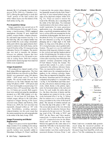
length). The second model (from here on computed and graphed in a stereoplot (Plot
referred to as the Video Model) was built 1 in Fig. 3). For both Photo and Video mod-
using 528 photos (3840 × 2160 pixels and els, the ρ direction is clustered along a great
4.77 mm focal length) extracted using VLC circle, which, thanks to the gimbal, repre-
software from a 257-second-long video file sents the horizontal plane in the real-world
(i.e., 2.6 frames per second). Both acquisi- frame. For each model, the entire data set
tions were carried out using the smartphone (i.e., the three directions of photos and the
mounted on a DJI OM4 gimbal, at a dis- four markers) are rotated to set the ρ great
tance of ~30 cm from the fault plane. To circle horizontal (Plot 2 in Fig. 3). Notice
include images oblique to the fault plane, that the rotation axis is univocally defined,
required to mitigate doming of the recon- being coincident to the strike of the best-fit
structed scene (James and Robson, 2014; plane. The amount of rotation instead can
Tavani et al., 2019), the view direction was be either the dip of the plane or 180° + dip. Figure 3. Lower hemisphere stereographic pro-
jection (stereonet) of the camera vectors for both
repeatedly changed within an ~60° wide The correct placement of the view direction the Photo and Video models, after model building
cone. Nevertheless, avoiding operator- (ξ) means that the selection between these (Plot 1), and after horizontalization of the ρ-vector
induced shadows into the scene meant that two options by the user is trivial. The result- great-circle envelope (Plot 2). In essence, after
this rotation, the vertical axis is paralleled to the
the main acquisition was sub-perpendicular ing trend of the CH strike is N211° and true vertical, but the azimuth is yet randomly ori-
to the strike of the fault, being ~ENE. N105° for the Photo and Video models, ented. (Plot 3) Stereonet of the camera vectors
after rotation around the vertical axis. (Plot 4)
respectively. A rotation about the vertical Rose diagram showing the distribution of the ρ
Image Processing and Model axis (57° counterclockwise for the Photo vectors in both models. CH—compass holder.
Registration Model and 49° clockwise for the Video
Images were processed in Agisoft Meta- Model) was applied to the entire data set to Point 2 and were eventually fully georefer-
shape (version 1.6.2), resulting in two unreg- match the CH strike to its measured value, enced using the measured position of
istered dense point clouds (Fig. 2C). Four i.e., N154° (Plot 3 in Fig. 3). The twice- Point 1. These two steps are achieved during
specific markers were manually added in rotated markers were then scaled using the the export stage from OpenPlot, which com-
Metashape. In Figure 2C, Point 1 and Point measured distance between Point 1 and piles a *.txt file containing the correctly
6 GSA Today | September 2021