Page 7 - i1052-5173-27-9

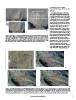
not imaged in A and B Case Study: Surprise Canyon,
Panamint Mountains, California, USA
A.
pixel Methods
smear
Terrestrial LiDAR survey (TLS) data
C. were acquired in Surprise Canyon in the
B. Panamint Mountains west of Death Valley
to conduct an experiment in 3D mapping.
Figure 3. Illustration of the power of using unmanned aerial system (UAS) imagery in Structure from Following that survey, we used a handheld,
Motion studies. Figure is a comparison of a near-vertical view of the same area developed using the GPS-enabled camera at sites of opportu-
same camera from ground-based images only (A and B) versus ground-level to ~100 m elevation nity and used the photographs to develop
UAS flight images (C). (A) is a visualization of the colored point cloud, whereas (B) is a textured SfM models that overlapped with the TLS
triangulated irregular network model, and (C) is a colored point cloud with all scenes processed at survey. The SfM data were co-registered
the same resolution using Agisoft PhotoScan. Seventy images were used in (A) and (B) versus 400 with the TLS data using a variety of
in (C), but the increase in resolution is primarily due to greater ranges of look angles in (C). ground control methods. Data acquisition
and error assessment for this study is con-
sidered elsewhere (Brush, 2015). The study
area was chosen because it contains com-
plex, metamorphic structures, arguably the
most challenging 3D visualization problem
in field studies, yet the area contains
superb bedrock exposures and significant
topographic relief. Thus, the site is nearly
ideal to test 3D mapping methods. SfM
models were generated using Agisoft
PhotoScan Professional software; Maptek’s
I-Site Studio was used to co-register SfM
and LiDAR point clouds as well as a 3D

N B.
A.

C. D.

Figure 4. Sequential development of the structural interpretation for the area in Figure 2D–2F. (A) shows field map at the end of the first season (one
field day) with contradictory interpretations. Yellow arrow shows view direction in Figure 2 and (B)–(D) in this figure. (B) shows an uninterpreted field
image captured on a tablet computer with the same image annotated in (C) showing the field interpretation after the second visit to the site versus the
final interpretation (D) developed from model interpretation and a field visit to confirm the interpretation. Linework in (A) shows form lines of layering
(green), main foliation (blue), inferred second cleavage (dashed thin red lines), intrusive contacts (magenta), and fault contacts (dashed red line).

www.geosociety.org/gsatoday 7