Page 6 - i1052-5173-32-9

spectrum. For example, in carbonate rocks at grain boundaries (Rogers and Kerr, 1942). contends with chromatic aberration, whereby
successive stages of calcite precipitation, Additionally, crossed polarizers in transmit- each wavelength of light achieves maximal
diagenesis, and recrystallization, differ- ted light setups heighten contrast between sharpness at a different focal depth due to the
ences in the trace element chemistry of features by creating differential extinction wavelength-dependence of light refraction
the stages will produce heterogeneities in and birefringence patterns (Rogers and Kerr, (Jacobson et al., 2013). In the supplemental
the strength of fluorescence and thus con- 1942). To image thin sections with transmit- material , we demonstrate how we apply blur
1
trast in the image (Dravis and Yurewicz, ted plane-polarized (PPL) and cross-polar- modeling and deconvolution to achieve
1985). Additionally, organic or apatitic fossil ized (XPL) light, we have created a light multispectral images that are sharper than a
materials often fluoresce, making UV fluo- table that can be used with GIRI or any cam- standard RGB camera.
rescence photography a valuable tool for cre- era stand setup (Fig. 1D). The light source for
ating contrast in paleontological samples this table is a dense Ramona Optics LED RESULTS
(Tischlinger and Arratia, 2013; Fig. 1B). To board with five wavelengths (470, 530, 620, In the following case studies, we illustrate
image fluorescence, we illuminate samples 850, 940 nm), which illuminates the sample two examples where the added spectral data
with a 365 nm SmartVision LED. To reduce through a diffuser and a broadband linear from our reflected and transmitted light set-
noise in the images, we place a bandpass fil- polarizer. To image XPL, we attach a second ups enhance our ability to distinguish fea-
ter with a cut-off wavelength of 395 nm over polarizer over the sample, perpendicular to tures within geological samples. To classify
the UV light to remove any visible compo- the lower linear polarizer (Fig. 1D). Unlike pixels, we use a support vector machine
nents of the emitted spectrum and use a 400 traditional petrographic microscopes, this (SVM), which is a simple machine learning
nm cut-on UV filter in front of the lens to light table holds the sample fixed, while a model, to show the potential for future
eliminate any UV light from reaching the NEMA 17 stepper motor rotates both polar- machine learning efforts when trained on
camera sensor. Note that when imaging with izers synchronously (Fueten, 1997) with a these more informative spectral data.
UV, the camera records the fluorescence of precision of 2.8 × 10 degrees.
−4
the materials in the VNIR spectrum. Case Study 1: Feature Mapping in
Data Processing Reflected Light
Transmitted Light In the case of both transmitted and A lack of contrast between classes in
Thin section transmitted light imagery reflected light, all captured image channels reflected light imagery commonly stems
offers another opportunity for increased con- are perfectly aligned, allowing the user to from all pixel values falling near a brightness
trast. Anisotropy, cleavage, and twinning view any three channels in a false color line—a 1:1 intensity line where values are
create distinctive qualities in grains and image or analyze all captures as a single mul- well-correlated between channels (Fig. 2B).
crystals within a thin section and delineate tichannel image. Our setup, like all cameras, In Figure 2A, we show an RGB image of an

A Red - Green - Blue 0.8 Pixel values D Red - Green - Blue
1
B
Green (530 nm) 0.6 Brightness
E,F
0.4
0.2
(TLS: 0.025)
0
0.5
Blue (470 nm) 1
1
C
0.6
1 mm UV - Yellow - Red Yellow (590 nm) 0.8 5.5875 UV - Yellow - Red
0.4
Dolomite Archaeocyath 0.2 Brightness E F
(TLS: 0.105)
Micrite Crack 0 0.5 1 R-G-B 65% accuracy UV-Y-R 91% accuracy
UV (365 nm)
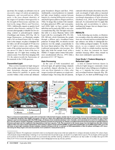
Figure 2. Improved segmentation results with multispectral reflected light imagery. (A) We take the same image of an archaeocyathid boundstone sample
in a traditional red-green-blue (RGB) colorspace, as well as a false color ultraviolet (UV)-yellow-red space and sample the same pixels for four feature
classes in each (colored boxes). (B) In the RGB image, all classes show covariance between color channels, and most pixels fall around the brightness line.
(C) In the UV-yellow-red (UV-Y-R) image, covariance between channels is removed for all classes, as evidenced by the fourfold increase in average distance
between each pixel and the brightness line (reported as total least squares, TLS). The movement of all classes away from the brightness line into distinct
regions of the color space eases segmentation. (D–F) Using a support vector machine (SVM), an automated classification of the RGB image is 65% accurate
and does not give high-resolution borders between classes and regions (D, E). In contrast, an SVM segmentation of the UV-yellow-red image is 91% accu-
rate and gives sharp region and class boundaries more suitable for measurements (D, F).

1 Supplemental Material. This supplement is intended to show our multispectral setup in more detail and explain how we mitigate chromatic aberration. We include a figure
with annotated computer-aided design renderings of our transmitted and reflected light setups, and details for our light emission spectra. The text begins with background
on the problem of chromatic aberration, details our experimental setup and blur modeling calculations, and discusses our final results. Go to https://doi.org/10.1130/
GSAT.S.19773532 to access the supplemental material; contact editing@geosociety.org with any questions.

6 GSA TODAY | September 2022